
Our recent arXiv posting of arXiv:1706.04191 "On the time lags of the LIGO signals" has generated considerable interest - both positive and negative. This is understandable given the significance of the claimed discovery of gravitational waves resulting from the merger of two black holes. In our opinion, a discovery of this importance merited a genuinely independent analysis of the data. It was the aim of our manuscript to perform such an analysis using publicly available data from LIGO and methods that were as close as possible to those adopted by the LIGO team. We focussed our attention mainly on the first event, GW150914, with special attention to the time lag between the arrival times of the signal at the Hanford and Livingston detectors. In our view, if we are to conclude reliably that this signal is due to a genuine astrophysical event, apart from chance-correlations, there should be no correlation between the "residual" time records from LIGO's two detectors in Hanford and Livingston. The residual records are defined as the difference between the cleaned records and the best GW template found by LIGO. Residual records should thus be dominated by noise, and they should show no correlations between Hanford and Livingston. Our investigation revealed that these residuals are, in fact, strongly correlated. Moreover, the time delay for these correlations coincides with the 6.9 ms time delay found for the putative GW signal itself.
As a member of the LIGO collaboration, Ian Harry states that he "tried to reproduce the results quoted in 'On the time lags of the LIGO signals'", but that he "[could] not reproduce the correlations claimed in section 3". Subsequent discussions with Ian Harry have revealed that this failure was due to several errors in his code. After necessary corrections were made, his script reproduces our results. His published version was subsequently updated. Regarding the results presented here, we also release a version of our script for comparison.
The process of separating signal and noise reliably is always difficult, but it is particularly challenging when the noise is neither gaussian nor stationary as in the present case. A thorough understanding of "cross talk" between the detectors is essential to ensure that cleaning techniques lead to reliable signal extraction. In the following we will describe a safe analysis based on publicly available LIGO data. This analysis will reveal a strong correlation between the Hanford and Livingston residuals.
We hope that interested people will repeat our calculations and will make up their own minds regarding the significance of the results. It is obvious that "belief" is never an alternative to "understanding" in physics.
The event GW150914 is characterized by its shape and its almost simultaneous appearance in the Hanford and Livingston detectors with a time lag of only $6.9$ ms. Here, we briefly review a method for confirming this time lag with the aid of cross-correlations to later apply it to the residual noise in the immediate vicinity of GW150914.
We denote the strain data, $H(t)$ and $L(t)$, within a given time interval $t_a\leq t\leq t_b$ as $H_{t_a}^{t_b}$, and $L_{t_a}^{t_b}$, respectively. Shifting a selected piece of Livingston data with respect to the Hanford data by a time lag $\tau$ allows for the calculation of the cross-correlation between the two records as a function of $\tau$. Due to the non-stationarity of the signal, we wish to only include values within a selected range, ensured by the method sketched below. Thus, our assumption is that within a sufficiently small time window the residuals behave in a stationary manner.
Using the scheme above, we define the cross-correlation coefficient as $$ C(t,\tau,w) = {\rm Corr}(H_{t+\tau_0 + \tau}^{t-\tau_0+\tau+w},L_{t+\tau_0}^{t-\tau_0+w}), $$ where $\tau_0$ is chosen to ensure that only values within the selected range $[t, t+w]$ are included. (We note that the GW150914 signal appeared first at the Livingston site and was seen at the Hanford site approximately $6.9$ ms later. Thus, the equation above has been written so that $\tau$ is positive for GW150914. We will restrict the time delay to $-10 \leq\tau\leq 10$ ms since this is the only region of physical interest for gravitational wave detection. Therefore we choose $\tau_0 = 10$ ms.) Here, ${\rm Corr}(x,y)$ is the standard Pearson cross-correlation function between records $x$ and $y$ defined to lie within the window, $w$: $$ {\rm Corr}(x_{t+\tau}^{t+\tau+w},y_{t}^{t+w}) = \frac{{\rm Cov}(x_{t+\tau}^{t+\tau+w},y_{t}^{t+w})}{\sqrt{{\rm Cov}(x_{t+\tau}^{t+\tau+w},x_{t+\tau}^{t+\tau+w}) \cdot {\rm Cov}(y_{t}^{t+w},y_{t}^{t+w})}}, $$ where ${\rm Cov}(x,y)$ is the usual covariance defined as ${\rm Cov}(x,y)=\langle (x-\langle x \rangle)(y - \langle y \rangle) \rangle$ and $\langle ... \rangle$ is the average within the window considered.
We begin our search for correlations in the residual noise with a simple cross-correlation test (hereafter CC-test) between Hanford and Livingston records using the data provided by the LIGO collaboration:
https://losc.ligo.org/s/events/GW150914/P150914/fig1-residual-H.txt
https://losc.ligo.org/s/events/GW150914/P150914/fig1-residual-L.txt
In the 0.2 s record including the GW event, the residual noise components in these records are calculated as $H_n=H-H_{\rm tpl}$ and $L_n=L-L_{\rm tpl}$.
Here, $H_{\rm tpl}$ and $L_{\rm tpl}$ are the templates cleaned in precisely the same manner as the raw data to yield the cleaned records, $H$ and $L$.
In order to highlight general properties of the cleaned GW150914 signal, the numerical relativity templates and the residuals, before turning to the CC-test, we show below the Fourier amplitudes for these various components for both Hanford and Livingston detectors, and briefly describe their peculiarities.
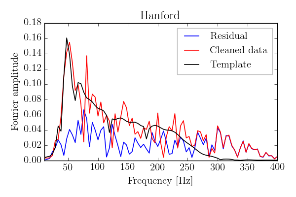
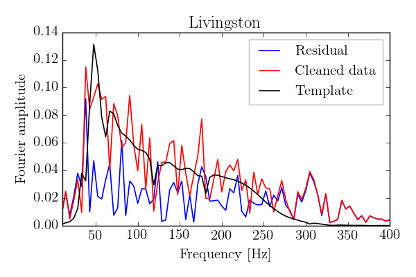
First, for both detectors, the templates and the cleaned data show a pronounced peak in the Fourier amplitudes near $50$ Hz that is associated with the band-pass filtering that selects the region of $35$ to $300$ Hz. Second, the amplitudes of the Hanford residuals decrease rapidly for $f<70$ Hz, while the Livingston residual amplitudes have a maximum value near $40$ Hz, which coincides with a peak in the cleaned record. Third, as is readily seen from the figures, for frequencies $f > 270$ Hz, the cleaned data is dominated by the residuals for both the H and L detectors. Moreover, we find amplitudes in the cleaned records that are substantially lower than those in the templates in, e.g. the frequency range $100 < f < 150$ Hz. It is especially worth to note this peculiarity in Hanford where the amplitudes of the cleaned data even fall below those of the residuals at frequencies around $70$ Hz and $120$ Hz. It should be kept in mind, however, that these "anomalies" describe properties of the residuals for the individual detectors and do not necessarily lead to cross-correlations between the H and L residuals. This "cross-talk" of these records is the subject of our paper and is summarized below.
The cross-correlation of $H_n$ and $L_n$ is calculated as a function of the time delay $\tau$. The constraint $|\tau|\le 10$ ms is dictated by the physical conditions for the arrival of a GW. All correlations are calculated in the time domain as described in the section above on cross-correlations, namely:
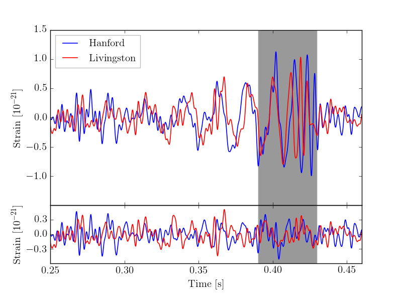
The figures below, equivalent to Fig. 7 in our paper, show the H and L time records and residuals after subtraction of the numerical relativity template. The left panel shows the original data, and the right panel shows the Livingston data shifted by 7 ms and inverted. The shaded area marks the range 0.39 to 0.43 seconds within which we compute the cross-correlation function presented below.


As seen, the calculation can be repeated for a variety of time intervals indicated in the legend. The figure reveals a surprisingly large cross correlation of $-0.81$ for the optimal window of 0.39 to 0.43 s. (The fact that this value is negative is a consquence of the fact that the Livingston signal should be inverted.) This is the region in which the "chirp" effect is most pronounced. We note that the cross-correlation between the Hanford and Livingston residuals has a magnitude greater than $0.12$ for the four ranges shown above. It is even more significant that a strong negative correlation is obtained for a time delay of approximately 7 ms for each of the time windows considered. While we did not further elaborate on this in our present paper, we will make investigations of significance the subject of a forthcoming study.
It should be noted that the template used here is the maximum-likelihood waveform. However, a family of such waveforms can be found that fit the data equally well. (See e.g. the panels in second row of Fig. 1 in LIGO's detection paper of GW150914.) In order to provide a rough estimate of this uncertainty, we have also explored the possibility of a free $\pm10\%$ scaling of the amplitude of the templates, so that $H_n=H-(1 \pm 0.1)H_{\rm tpl}$ and $L_n=L-(1 \pm 0.1)L_{\rm tpl}$. (This crude estimate of the uncertainties will obviously change both the magnitudes and phases of the Fourier amplitudes of the residuals.) The resulting cross correlations are virtually identical to the results shown above. Given that the residual noise is significantly greater than the uncertainty introduced by the family of templates, this is result is not surprising.
It would appear that the 7 ms time delay associated with the GW150914 signal is also an intrinsic property of the noise. The purpose in having two independent detectors is precisely to ensure that, after sufficient cleaning, the only genuine correlations between them will be due to gravitational wave effects. The results presented here suggest this level of cleaning has not yet been obtained and that the identification of the GW events needs to be re-evaluated with a more careful consideration of noise properties.
We hope that our comment will improve the undestanding of the major results in our paper. We are thankful to Alessandra Buonanno and Ian Harry for scientific discussions, and for making their Python script available to us and the scientific community.